
- What is statistical process control
- SPC visual map
- Origins: from Shewhart to Japanese industry
- Common cause vs. special cause variation
- Which control chart to use
- How to calculate X-bar and R chart limits
- Reading the chart: special cause signals
- How to implement SPC step by step
- Industrial examples
- Stability first, capability second
- Common mistakes
- Benefits
- Implementation checklist
- Frequently asked questions
What is statistical process control
Every process varies. Two shafts machined on the same lathe, by the same operator, with the same program, never come out with exactly the same diameter. Statistical process control (SPC) puts that variation to work: instead of finding problems at final inspection, the team watches the process while it runs and reacts when its behavior changes.
The core SPC tool is the control chart: a plot of a measurement over time with a center line and two limits calculated from the process's own data. Points inside the limits with no pattern mean a stable process. A point outside, or a suspicious run, means something has changed and deserves attention before it becomes scrap.
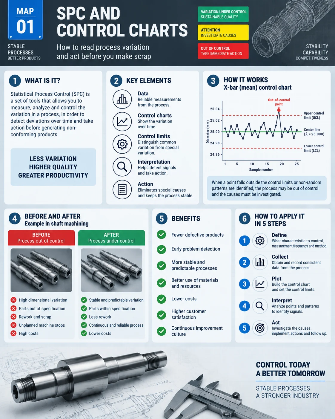
SPC visual map
The map below sums up the concept, the key elements, an X-bar chart with a special cause signal, a before and after from a machining cell and the rollout steps. Feel free to download it for training sessions and team boards.
Origins: from Shewhart to Japanese industry
Walter A. Shewhart proposed the control chart in the 1920s while working in the Bell System in the United States. According to the NIST/SEMATECH e-Handbook of Statistical Methods, Shewhart's model sets the center line and the limits from the mean and standard deviation of the plotted statistic. The idea behind it is simple: separate the variation built into the system from variation that has an assignable cause.
W. Edwards Deming took these ideas to Japan after the war, and statistical control became part of the quality foundation of Japanese manufacturing. Today SPC shows up in automotive customer requirements, in the Control phase of Six Sigma DMAIC and in any plant that must prove its process is predictable.
Common cause vs. special cause variation
| Common cause | Special cause | |
|---|---|---|
| What it is | Natural variation of the system: small differences in material, temperature, normal wear | Event with an assignable cause: broken tool, off-spec material lot, edited program |
| How often | Always present | Sporadic |
| On the chart | Points inside the limits, no pattern | Point beyond a limit or a non-random pattern |
| Who acts | Management, by changing the system (machine, method, design) | The workstation, right away, following the reaction plan |
Mixing them up is the costliest mistake in SPC. Adjusting the machine after every small natural swing, what Deming called tampering, increases variation instead of reducing it. Ignoring a special cause signal lets the problem keep making scrap until someone notices.
Which control chart to use
| Chart | When to use it | Data type |
|---|---|---|
| X-bar and R | Small subgroups, from 2 to about 10 parts | Variables (measurements) |
| X-bar and S | Larger subgroups | Variables |
| I-MR (individuals) | One reading at a time: a chemical batch, oven temperature | Variables |
| p | Fraction defective, variable sample size | Attributes |
| np | Number of defective units, fixed sample size | Attributes |
| c | Defects per unit, constant inspection area | Attributes |
| u | Defects per unit, variable sample size | Attributes |
Measurements carry more information than pass or fail data. Whenever a characteristic can be measured, use a variables chart: it detects shifts sooner and with smaller samples.
How to calculate X-bar and R chart limits
Example: a cell machines shafts with a 25.00 mm nominal diameter. Every hour the operator measures 5 consecutive parts (subgroup size n = 5). After 20 subgroups, the grand average is X̿ = 25.000 mm and the average range is R̄ = 0.050 mm.
X-bar chart: UCL = X̿ + A₂·R̄ | CL = X̿ | LCL = X̿ − A₂·R̄
R chart: UCL = D₄·R̄ | CL = R̄ | LCL = D₃·R̄
| n | A₂ | D₃ | D₄ | d₂ |
|---|---|---|---|---|
| 2 | 1.880 | 0 | 3.267 | 1.128 |
| 3 | 1.023 | 0 | 2.574 | 1.693 |
| 4 | 0.729 | 0 | 2.282 | 2.059 |
| 5 | 0.577 | 0 | 2.114 | 2.326 |
With n = 5, the X-bar UCL is 25.000 + 0.577 × 0.050 = 25.029 mm and the LCL is 24.971 mm. On the R chart, UCL = 2.114 × 0.050 = 0.106 mm and LCL = 0.
Control limits are not specification limits. Control limits are the voice of the process, calculated from data. Specification limits are the voice of the customer, taken from the drawing. A process can be in control and still make parts out of tolerance, and the reverse also happens.
Source: NIST/SEMATECH, Shewhart X-bar and R and S Control Charts.
Reading the chart: special cause signals
A point beyond the limits is the best-known signal, but not the only one. The Western Electric rules, presented by NIST, split the chart into 1, 2 and 3 sigma zones and flag:
- 1 point beyond 3 sigma, outside the UCL or LCL.
- 2 out of 3 consecutive points beyond 2 sigma, on the same side.
- 4 out of 5 consecutive points beyond 1 sigma, on the same side.
- 8 consecutive points on the same side of the center line.
More rules mean more false alarms. Pick a set, write it into the procedure and stick with it.
When a signal appears, the operator follows the station's reaction plan: quarantine everything made since the last good subgroup, call the team leader, find the cause (the 5 Whys help) and record it in the chart's event log. It is the same spirit as jidoka: stop at the first sign so no defect moves downstream.
Source: NIST/SEMATECH, What are Variables Control Charts?.
How to implement SPC step by step
- Pick a few critical characteristics, the ones customers feel or that drive the most scrap. Starting with dozens of charts is the fastest way to turn SPC into paperwork.
- Validate the measurement system. If the gauge varies almost as much as the process, the chart ends up measuring the gauge. A gauge R&R study settles it.
- Define rational subgroups and frequency: consecutive parts taken together, often enough to catch a shift before it becomes a lost batch.
- Collect 20 to 25 subgroups, calculate the limits and check stability. If special causes show up in that period, investigate, remove them and recalculate.
- Train operators to measure, plot and react. The chart lives at the workstation as part of visual management.
- Revise limits only when the process truly changes, for example after a proven improvement.
Industrial examples
- Machining: diameter and length on X-bar and R charts, one subgroup per hour or per tool change.
- Food and cosmetics filling: net weight on X-bar and S charts, to avoid overfilling (cost) and underfilling (complaints and fines).
- Injection molding: fraction of parts with flash or short shots on a p chart, per shift.
- Automotive assembly: fastening torque on an I-MR chart when each reading comes from a data-logging nutrunner.
- Painting: defects per painted part on a c or u chart.
Stability first, capability second
Capability only makes sense for a stable process. With the chart in control, sigma can be estimated as σ = R̄ / d₂. In the example, σ = 0.050 / 2.326 ≈ 0.0215 mm. If the shaft specification is 25.00 ± 0.10 mm:
Cp = (USL − LSL) / 6σ = 0.20 / 0.129 ≈ 1.55
Cpk = min[(USL − mean) / 3σ, (mean − LSL) / 3σ]
With the process centered at 25.000, Cpk is also about 1.55. If the mean drifts to 25.05, Cp stays the same but Cpk drops to about 0.78, because the process is crowding the upper limit. Customers commonly require a minimum Cpk of 1.33, with higher values for critical characteristics or initial studies; always check the customer's requirement.
Common mistakes
- Drawing specification limits instead of control limits.
- Adjusting the machine after every point, reacting to common cause variation.
- Filling in the chart at the end of the shift, just for the audit.
- Recalculating limits every week, which hides slow drift.
- Charts with no reaction plan: the operator sees the signal and doesn't know what to do.
- Measuring with an unvalidated gauge.
Benefits
- Less scrap and rework, because shifts show up before they become batches.
- Less reliance on final inspection: quality is controlled at the source.
- Data-driven decisions: the chart shows when to act and, just as important, when to leave the process alone.
- A reliable basis for capability studies and improvement projects.
- Operators with ownership of their own station's quality.
Implementation checklist
- Critical characteristic selected and justified.
- Measurement system validated.
- Subgroup size and frequency defined.
- Limits based on 20 to 25 stable subgroups.
- Reaction plan written and trained.
- Chart at the workstation, filled in at the time of measurement.
- Event log with the special causes found.
- Regular review by leaders at the gemba.
Frequently asked questions
What does SPC stand for?
Statistical process control: using statistical tools, mainly the control chart, to monitor a process and separate natural variation from special causes.
What is the difference between control limits and specification limits?
Control limits are calculated from process data and show what the process can do. Specification limits come from the customer or the drawing and show what is acceptable.
How many subgroups do I need to set control limits?
The usual practice is 20 to 25 subgroups from a stable process before fixing the limits.
When should I use a p chart instead of an X-bar and R chart?
When the data are attributes, such as good or bad parts. If the characteristic can be measured, an X-bar and R chart detects shifts sooner.
Is SPC the same as Six Sigma?
No. SPC is a monitoring tool; Six Sigma is an improvement project methodology that uses SPC in the Control phase of DMAIC.
Sources
- NIST/SEMATECH e-Handbook of Statistical Methods. What are Variables Control Charts? https://www.itl.nist.gov/div898/handbook/pmc/section3/pmc32.htm
- NIST/SEMATECH e-Handbook of Statistical Methods. Shewhart X-bar and R and S Control Charts. https://www.itl.nist.gov/div898/handbook/pmc/section3/pmc321.htm
- MONTGOMERY, D. C. Introduction to Statistical Quality Control. Hoboken: Wiley.
Found a special cause? Solve it at the root.
Download the free "Problem Solving Kit" e-book, with PDCA, A3, 5 Whys and Ishikawa.
Download the e-book
About the author
Lean Manufacturing & Behavioral Management Specialist
Over 20 years in the automotive and metalworking industries (GM and Dana), Lean Manufacturing practitioner since 2006. SENAI instructor and mentor in Brazil’s Brasil Mais Produtivo program, delivering consulting, training and audits for 50+ companies, combining quality, productivity and people development.