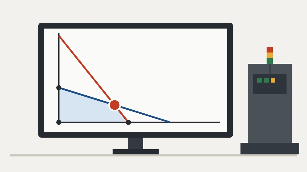
What linear programming is
Linear programming is an optimization technique that finds the best value, maximum or minimum, of an objective function subject to a set of linear constraints. In manufacturing it answers questions like: how much of each product should we make to earn the highest margin with the machine and labor hours we have?
The simplex method, created by George Dantzig in 1947, is the algorithm that solves these problems by moving along the corner points of the feasible region until it reaches the optimum.
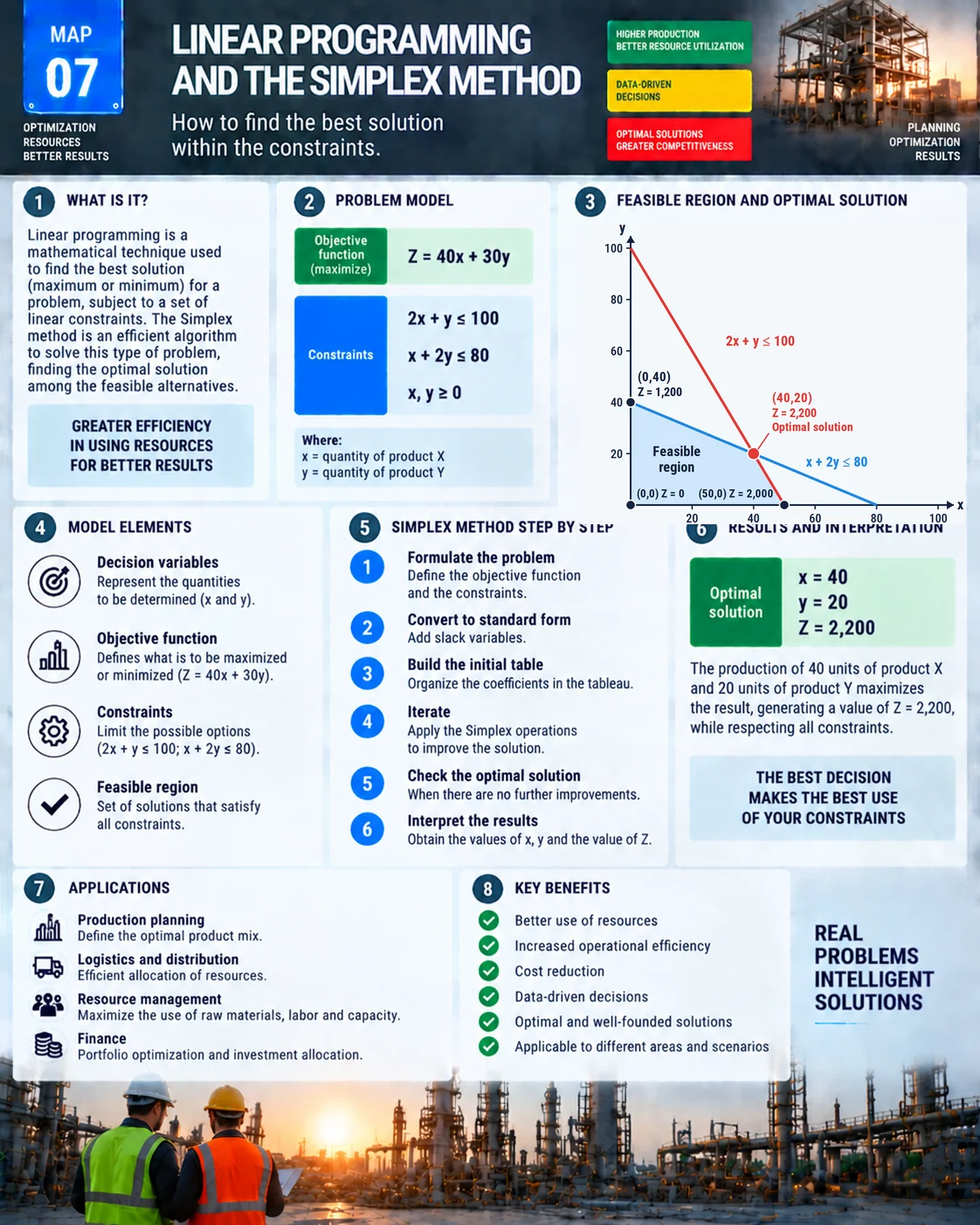
Linear programming visual map
The map shows the model elements, the feasible region with its four corner points, the optimal solution and the simplex steps.
Model elements
| Element | Meaning | In the example |
|---|---|---|
| Decision variables | What we want to determine | x = units of product A; y = units of product B |
| Objective function | What we want to maximize or minimize | Z = 40x + 30y (total margin) |
| Constraints | Resource limits | 2x + y ≤ 100 and x + 2y ≤ 80 |
| Non-negativity | No negative production | x ≥ 0 and y ≥ 0 |
| Feasible region | Points that satisfy every constraint | Polygon with corners (0,0), (50,0), (40,20) and (0,40) |
Example: a two-product mix
Each unit of A earns a margin of 40 and each unit of B earns 30. The first constraint can stand for machine hours (A uses 2 hours, B uses 1, 100 are available); the second for assembly hours (A uses 1, B uses 2, 80 are available).
Maximize Z = 40x + 30y | 2x + y ≤ 100 | x + 2y ≤ 80 | x, y ≥ 0
Graphical method: check the corner points
With two variables you can draw the constraints and see the feasible region. The optimum always sits at a corner point:
| Corner (x, y) | Z = 40x + 30y | Note |
|---|---|---|
| (0, 0) | 0 | Origin |
| (50, 0) | 2,000 | Product A only |
| (0, 40) | 1,200 | Product B only |
| (40, 20) | 2,200 | Intersection of both constraints: optimum |
The optimal solution is to make 40 units of A and 20 of B, for Z = 2,200. At that point both constraints are binding: 2 × 40 + 20 = 100 and 40 + 2 × 20 = 80.
How the simplex method reaches the same answer
- Formulate the problem: objective function and constraints.
- Convert to standard form: add slack variables (2x + y + s1 = 100; x + 2y + s2 = 80).
- Build the initial tableau, starting at the origin.
- Iterate: the variable that improves Z the most enters the basis and the one that hits its limit first leaves.
- Check optimality: when no variable can improve Z, the solution is optimal.
- Interpret: x = 40, y = 20, zero slack and Z = 2,200.
Nobody builds tableaus by hand for real problems: Excel Solver with the Simplex LP engine handles hundreds of variables in seconds.
Shadow prices: what one more hour is worth
Sensitivity analysis shows how much Z improves when a constraint is relaxed. In the example, one more machine hour raises Z by about 16.67, and one more assembly hour by about 6.67. These shadow prices show where to invest: adding machine capacity pays more than adding assembly capacity, as long as the extra hour costs less than the gain.
The same logic appears in the Theory of Constraints: the resource with the highest shadow price is the economic bottleneck.
Applications
- Production planning: optimal product mix, as in the example, supporting production planning and control.
- Cutting stock: least waste when cutting sheets, coils and bars.
- Logistics: lowest-cost transportation and load allocation.
- Blending: feed, alloys and fuels at the lowest cost while meeting specifications.
- Staff scheduling and resource allocation.
Common mistakes
- A badly modeled objective function that mixes revenue and margin.
- Missing constraints that produce solutions the shop floor cannot run.
- Inequality signs reversed (≤ instead of ≥).
- Ignoring that variables must be whole numbers for parts; use integer programming in that case.
- Applying the result without checking that it makes sense to the people running the operation.
Frequently asked questions
What is linear programming?
An optimization technique that maximizes or minimizes a linear function subject to linear constraints, such as limited resources.
What is the simplex method?
The algorithm created by George Dantzig that moves along the corner points of the feasible region until it finds the optimal solution.
What is the solution to the example?
Make 40 units of A and 20 of B, for Z = 2,200, at the corner where both constraints intersect.
How do you solve linear programming in Excel?
Use the Solver add-in: set the objective cell, the variable cells and the constraints, then choose the Simplex LP method.
What is a shadow price?
How much the objective function improves with one more unit of a limited resource.
Sources
- DANTZIG, G. B. Linear Programming and Extensions. Princeton: Princeton University Press, 1963.
- HILLIER, F. S.; LIEBERMAN, G. J. Introduction to Operations Research. New York: McGraw-Hill.
- TAHA, H. A. Operations Research: An Introduction. Hoboken: Pearson.
Want to decide with numbers?
Download the free metrics e-book for production management.
Download the e-book
About the author
Lean Manufacturing & Behavioral Management Specialist
Over 20 years in the automotive and metalworking industries (GM and Dana), Lean Manufacturing practitioner since 2006. SENAI instructor and mentor in Brazil’s Brasil Mais Produtivo program, delivering consulting, training and audits for 50+ companies, combining quality, productivity and people development.